Coding for OSINT Data Analysis (for beginners): Part 1

This post is for absolute beginners and will train the reader in how to do introductory data analysis using Python and SQL coding languages, and the Google Colab tool.

To get started with SQL in Google Colab and practice some data analysis techniques, you can follow these steps:

Step 1: Setting Up SQL in Google Colab

Google Colab doesn’t come with SQL installed by default, but we can use SQLite, a lightweight database that runs within Colab. Here’s how to set it up:

1. Open a New Google Colab Notebook (https://colab.research.google.com/), click on New Notebook. Start entering your code where it says “start coding”. This is a coding cell. To create a new coding cell, click where it says “+ Code”, but you don’t have to do that just yet.

   

2. Install SQLite if it’s not already available by typing the following Python command in the cell:

import sqlite3

3. Run the cell by pressing Shift + Enter or clicking the Run button that looks like an arrow on the left side of the cell.

Background Info: when you open a new Google Colab notebook, it automatically defaults to using Python, so you don’t need to specify the language. You can type import sqlite3 directly in a code cell and press Shift + Enter (or just click the "Run" button) to execute it. This will import the SQLite library, enabling you to use SQL within Python.

---

I’m excited to announce the release of my new book,
Cryptocurrency Investigations: A Step-by-Step Guide to Tracing Digital Assets and Tracking Down Their Owners. Check it out on Amazon: https://www.amazon.com/dp/B0DJ1BN7ZM

This comprehensive guide is designed to help investigators, analysts, and anyone interested in the crypto space navigate the complexities of tracing digital assets and uncovering the identities behind them. Whether you’re new to crypto or a seasoned investigator, I hope you’ll find valuable insights and practical strategies inside.

---

Step 2: Creating a Database and Loading Data in SQLite

1. Create an In-Memory Database

   • SQLite lets you create an in-memory database, which only exists while your notebook is running. This is useful for temporary testing.

   • You start by connecting to this in-memory database with sqlite3.connect(':memory:').

import sqlite3

# Connect to an in-memory SQLite database

conn = sqlite3.connect(':memory:')

cursor = conn.cursor() # Create a cursor to execute SQL commands

• Here, conn represents the connection to your database, and cursor is the object you’ll use to run SQL commands.

2. Create a Table

• In SQL, a table is a structure for storing data with columns for each data type. Let’s create a simple table called employees with columns for id, name, age, department, and salary.

# Create an 'employees' table with columns for id, name, age, department, and salary

cursor.execute('''

CREATE TABLE employees (

id INTEGER PRIMARY KEY,

name TEXT,

age INTEGER,

department TEXT,

salary REAL

)

''')

(Also note that the numbers in the top left between brackets, like [2], is autogenerated. You do not type that in with your code. )

• Here, CREATE TABLE is the SQL command that tells SQLite to make a new table named employees.

• Each column is defined with a name and data type:

  • id is an INTEGER PRIMARY KEY, which uniquely identifies each row.

  • name is TEXT (text data).

  • age is an INTEGER.

  • department is TEXT.

  • salary is a REAL number (decimal).

  3. Insert Sample Data

  • Now that the table is ready, you can insert some sample rows. We’ll use INSERT INTO to add data to the employees table.

# Insert sample data into the employees table

cursor.executemany('''

INSERT INTO employees (name, age, department, salary)

VALUES (?, ?, ?, ?)

''', [

('Alice', 30, 'HR', 50000),

('Bob', 24, 'Engineering', 60000),

('Carol', 27, 'Sales', 45000),

('Dave', 35, 'Engineering', 70000)

])

• cursor.executemany allows you to insert multiple rows at once.

• Each tuple in the list represents a row of data (e.g., ('Alice', 30, 'HR', 50000)).

• The ? symbols are placeholders for the values in each tuple.

4. Commit the Changes

• SQLite requires you to commit changes to save them to the database. This isn’t strictly necessary with an in-memory database, but it’s a good habit.

conn.commit() # Save (commit) the changes

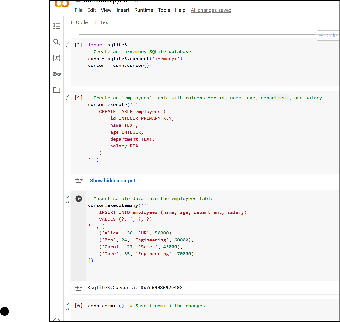
So at this point your screen looks like this:

Background Info: What Does it Mean to "Commit" Changes?

In databases, "committing" means permanently saving any changes you’ve made (like adding, updating, or deleting records). Until you commit:

• The changes exist only temporarily, and you can undo them if you need to.

• If you’re using a database stored on disk (not in-memory), uncommitted changes would be lost if you closed the connection.

In SQLite, especially with an in-memory database (like ':memory:'), the commit is less critical because everything exists temporarily while the program is running. However, it’s a best practice to commit changes whenever you modify data (insert, update, delete) to ensure those changes are saved.

Here’s the command we use:

conn.commit() # Saves changes

5. Displaying Data to Confirm It Worked

You can display the data to confirm everything is set up correctly. Use a SELECT query to retrieve data from the employees table and print it out. Here’s how:

# Query all rows from the employees table

cursor.execute('SELECT * FROM employees')

rows = cursor.fetchall() # Fetch all results

# Display results

for row in rows:

print(row)

This code does the following:

• cursor.execute('SELECT * FROM employees') runs a SQL query to get all records from the employees table.

• fetchall() retrieves all results of the query and stores them in rows.

• Finally, we print each row to see the data.

Using Pandas for Display

You can also display the data in a more readable table format using the pandas library:

import pandas as pd

# Load data into a Pandas DataFrame

df = pd.read_sql_query('SELECT * FROM employees', conn)

df # Display the DataFrame in a table format

This will display the table directly in Google Colab in a familiar spreadsheet-style format, making it easy to confirm that your data was inserted correctly.

Step 3: Basic SQL Data Analysis Techniques

Once you have data in your SQLite database, you can try some SQL-based analysis techniques.

• Aggregations: Use SQL functions like COUNT, SUM, AVG, MIN, and MAX for basic descriptive statistics.

# Calculate the average salary

cursor.execute('SELECT AVG(salary) FROM employees')

avg_salary = cursor.fetchone()[0]

print('Average Salary:', avg_salary)

• Grouping: GROUP BY is useful for analyzing data across categories. For example, finding the average salary by department:

cursor.execute('SELECT department, AVG(salary) FROM employees GROUP BY department')

rows = cursor.fetchall()

for row in rows:

print(row)

• Filtering: WHERE clauses can help filter data, such as finding employees older than 25:

cursor.execute('SELECT name FROM employees WHERE age > 25')

rows = cursor.fetchall()

for row in rows:

print(row[0])

• Sorting: Use ORDER BY to sort results, such as listing employees by salary in descending order:

cursor.execute('SELECT name, salary FROM employees ORDER BY salary DESC')

rows = cursor.fetchall()

for row in rows:

print(row)

Step 4. Exporting Results

After analyzing your data, you may want to export it to a DataFrame for visualization in Colab. This is basically what we did earlier, but lets review anyhow.

import pandas as pd

# Load SQL query results into a DataFrame

df = pd.read_sql_query('SELECT * FROM employees', conn)

print(df)

In the next Data Analysis post we will address how to work with large data sets.

That’s all for now.